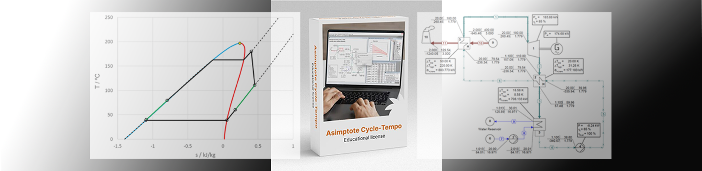
A new series of model examples has been added to the Cycle-Tempo model examples on the website, consisting of a simple organic subcritical Rankine cycle system and a recuperated one. No effort has been done to present optimal systems in terms of efficiency, performance, and costs; this example is just to show how you can model ORC system in Cycle-Tempo.
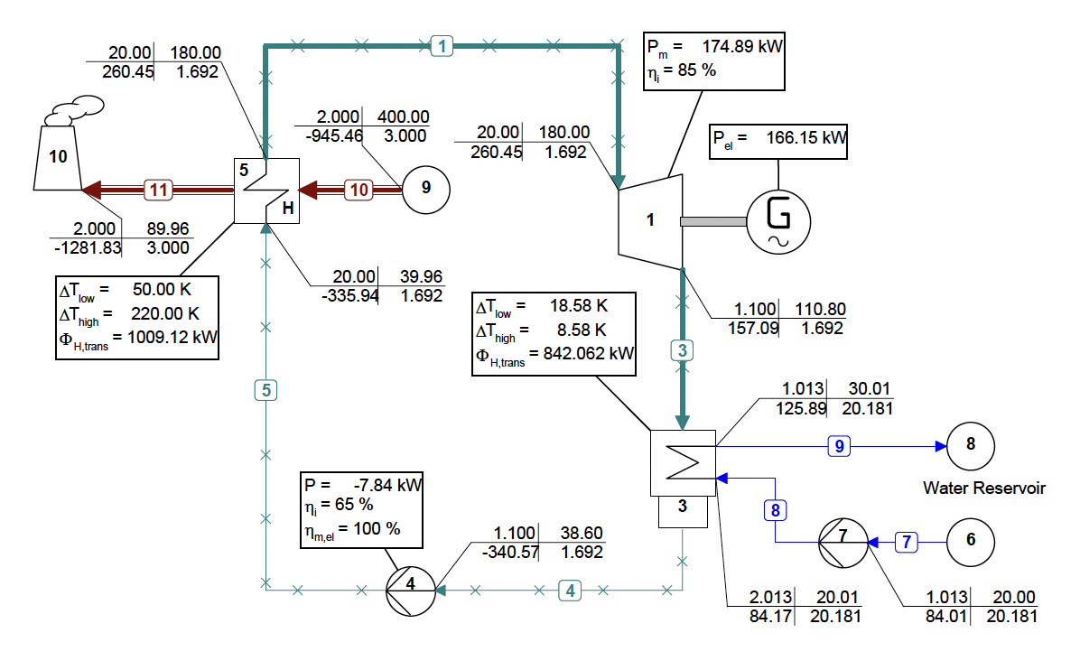
Assumptions are an energy supply by hot flue gases: pressure = 2 bar, temperature = 400 °C, mass flow = 3 kg/s, turbine inlet conditions temperature = 180 °C and pressure = 20 bar, and a water-cooled super atmospheric condenser with cooling water inlet temperature of 20 °C.
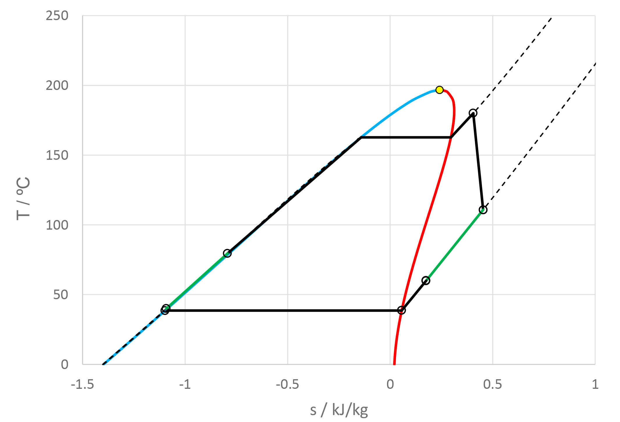
As working fluid, the hydrocarbon n-pentane is selected because it has an evaporation temperature of 162.7 °C at 20 bar and a condensation temperature of about 38.6 °C at 1.1 bar. The critical temperature is 196.6 °C and the critical pressure 33.7 bar. All fluid data are according to the freeStanMix model in FluidProp.
A Cycle-Tempo process scheme is presented in the figure below.
Cycle-Tempo does not support state diagrams for other fluids than water/steam (yet). Therefore, we used an Excel spreadsheet to visualize the system behavior in a temperature-entropy (T-s) chart. It is easy to draw the saturation lines and some isobars of a fluid in a T-s chart using FluidProp. Next, it is little bit more work, we copy the data of the table “Data for all pipes” in the Cycle-Tempo output and paste it directly in Excel and making use of these data we connect the state points in the T-s chart. Once setup, next time, data for different conditions can be copied and pasted and the results are immediately visible in Excel.
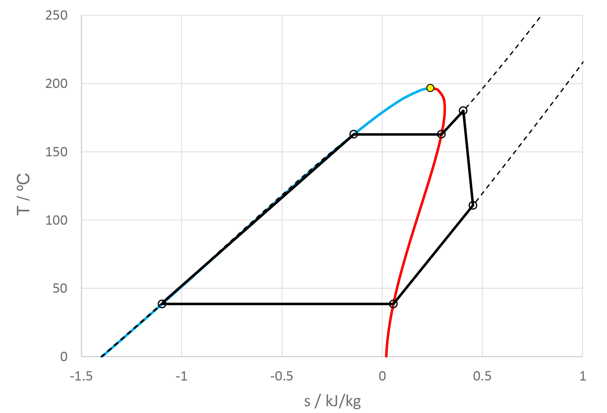
In the figure above, a T-s chart created in this way is depicted. From this figure one can notice that the condenser has to do quite some cooling before condensation takes place. Therefore, it can be concluded that the use of recuperator (regenerator) might be justified (in terms of performance and efficiency). In the figure below a Cycle-Tempo scheme is presented of a similar system but then including a recuperator.
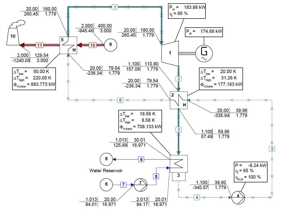
Immediately it is clear that the performance of the system increases from 166 kW to 175 kW, which is almost 5.5 %. An Excel sheet is created for this system by copying the previous one and extending the data with data for the recuperator. In the following figure, the T-s chart is presented.
The green lines of the process in the T-s chart indicate the amount of heat the recuperator regenerates. As a result, the boiler/evaporator now just has to heat the working fluid only from 80 °C instead of 40 °C in case of the first version, the simple ORC system.
As stated before, this example is just to present a way to model an ORC system in Cycle-Tempo and to show a way to visualize some of the results in a T-s chart in Excel. Although n-pentane is relatively greenhouse-friendly working fluid, other fluids are also possible, probably even performing better in terms of power output. In FluidProp and as a consequence also in Cycle-Tempo, several refrigerants (also modern ones with a with a low global warming potential, for example) are available to potentially do the same job, overcoming the issue of flammability of hydrocarbons. Furthermore, mixtures of working fluids are also possible.
In Cycle-Tempo, ORC systems can be developed for several temperature levels, for example lower temperature geothermal systems, systems for automotive applications, and solar powered systems. For condensers an air-cooled type might be a choice. Higher working fluid temperatures are possible using siloxanes, which are usually more stable at higher temperatures than hydrocarbons (like n-pentane) and refrigerants. At last, aside from subcritical systems as in this example, also supercritical systems are possible.
You can download the Cycle-Tempo files of these ORC systems here.